Learnings from optimising 22 of our most expensive Snowflake pipelines

We recently spent a sprint focused on reducing our Snowflake costs. During this sprint, we investigated 22 of our most expensive pipelines (in terms of Snowflake costs), one by one. In total we merged 56 changes, and in this post we’ll be laying out the optimisations that worked best for us.

Most of these changes were just common sense and didn’t involve any advanced data engineering techniques. Still, we’re always making mistakes (and that’s okay!) and hopefully this post will help readers avoid a few of the pitfalls we encountered.

⚠️ Medium is now 14 years old. Our team has inherited a tech stack that has a long history, some flaws and technical debt. Our approach to this problem was pragmatic; we’re not trying to suggest big pipeline re-designs to reach a perfect state, but rather consider our tech stack in it’s current state and figure out the best options to cut costs quickly. Our product evolves, and as we create new things we can remove some old ones, which is why we don’t need to spend too much time re-factoring old pipelines. We know we’ll rebuild those from scratch at some point with new requirements, better designs and more consideration for costs and scale.

Do we need this?

In a legacy system, there often are some old services that just “sound deprecated.” For example, we have a pipeline called medium_opportunities , which I had never heard about in 3 years at Medium. After all, it was last modified in 2020… For each of those suspect pipelines we went through a few questions:

• Do we need this at all?? Through our investigation, we did find a few pipelines that were costing us more than $1k/month and that were used by… nothing.
• A lot of our Snowflake pipelines will simply run a Snowflake query and overwrite a Snowflake table with the results. For those, the question is: Do we need all of the columns? For pipelines we cannot delete, we identified the columns that were never used by downstream services and started removing them. In some cases, this removed the most expensive bottlenecks and cut the costs in a massive way.
• If it turns out the expensive part of your pipeline is needed for some feature, you should question if that feature is really worth the cost or if there is a way to tradeoff some cost with downgrading the feature without impacting it too much. (Of course, there are situations where it’s just an expensive and necessary feature…)
• Is the pipeline schedule aligned with our needs? In our investigation we were able to save a bunch of money just by moving some pipelines from running hourly to daily.

An example:

A common workflow among our pipelines involves computing analytics data in Snowflake and exporting it to transactional SQL databases on a schedule. One such pipeline was running on a daily schedule to support a feature of our internal admin tool. Specifically, it gave some statistics on every user’s reading interests (which we sometimes use when users complain about their recommendations).

It turns out this was quite wasteful since this feature wasn’t used daily by the small team who relies on it (maybe a couple times per week). So, we figured we could do away with the pipeline and the feature, and replace it with an on-demand dashboard in our data visualization tool. Then the data will be computed only when needed for a specific user. It might require the end user to wait a few minutes for the data, but it’s massively cheaper because we only pay when somebody triggers a query. It’s also less code to maintain and a data viz dashboard is much easier to update and adapt to our team’s needs.

Old vs new architecture for this example

To conclude this section, here are a few takeaways that I think you can activate right away at your company:

• Make sure your analytics tool has a way to sync with Github. Our data scientist gustavo set that up for us with Mode and it has been massively helpful to quickly identify if tables are used in our data visualisations.
• Make sure you document each pipeline. Just one or two lines can save hours for the engineers who will be looking at this in 4 years like it’s an ancient artifact. I can’t tell you the amount of old code we find every week with zero docs and no description or comments in the initial PR 🤦
• Deprecate things as soon as you can. If you migrate something, the follow-up PRs to remove the old code and pipelines should be part of the project planning from the start!
• Avoid select * statements as much as possible. Those make it hard to track which columns are still in-use and which ones can be removed without downstream effects.

Filtering is key

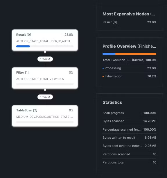
By using Snowflake Query Profile we were able to drill down on each pipeline and find the expensive table scans in our queries. (We’ll publish another blog post about the tools we used for this project later on). Snowflake is extremely efficient at pruning queries and that’s something we had to leverage to keep our costs down. We’ve found many examples where the data was eventually filtered out from the query, but Snowflake was still scanning the entire table. So if we have one key piece of advice here, it’s that the filtering should be very explicit in order to make it easier for Snowflake to apply the pruning.

Snowflake’s query profile tool

Sometimes Snowflake needs a tip

Here’s an example: Let’s say that we want to get the top 30 posts published in the last 30 days that got the most views in the first 7 days after being published. Here’s a simple query that would do this:

select post_id, count(*) as n_views
from events
       join posts using (post_id)
-- only look at view events
where event_name = 'post.clientViewed'
  -- only look at views on the first seven days after publication
  and events.created_at between to_timestamp(posts.first_published_at, 3) and to_timestamp(posts.first_published_at, 3) + interval '7 days'
  -- only look at posts published in the last 30 days
  and to_timestamp(posts.first_published_at, 3) > current_timestamp - interval '30 days'
group by post_id
order by n_views desc
limit 30

If we look at the query profile we can see that 11% of the partitions from the events table were scanned. That’s more than expected. It seems like Snowflake didn’t figure out that it can filter out all the events that are older than 30 days.

Let’s see what happens if we help Snowflake a little bit:

Here I’m adding a mathematically redundant condition: events.created_at > current_timestamp — interval ’30 days’ . Mathematically, we don’t need this condition because created_at ≥ published_at ≥ current_timestamp -interval ’30 days’ ⇒ created_at ≥ current_timestamp — interval ’30 days’ .

select post_id, count(*) as n_views
from events
       join posts using (post_id)
-- only look at view events
where event_name = 'post.clientViewed'
  -- only look at views on the first seven days after publication
  and events.created_at between to_timestamp(posts.first_published_at, 3) and to_timestamp(posts.first_published_at, 3) + interval '7 days'
  -- only look at posts published in the last 30 days
  and to_timestamp(posts.first_published_at, 3) > current_timestamp - interval '30 days'
  -- mathematically doesn't change anything
  and events.created_at > current_timestamp - interval '30 days'
group by post_id
order by n_views desc
limit 30

Still, this helps Snowflake a bunch and we’re now only scanning 0.5% of our massive events table and the overall query is now 5 times faster to run!

Simplify your predicates

Here’s another example where you can help Snowflake optimise pruning.

If you have some complex predicates in your filtering rule, Snowflake may have to scan and evaluate all of the rows although that could be avoided with pruning.

The following query scans 100% of the partitions in our posts table:

select *
from posts
-- only posts published in the last 7 days
-- (That's an odd way to write it, I know.
-- This is to illustrate how predicates can impact performance) 
where datediff('hours', to_timestamp(published_at, 3), current_timestamp - interval '7 days') > 0

If you simplify this just a little bit, Snowflake will be able to understand that partition pruning is possible:

select *
from posts
-- only posts published in the last 7 days
where to_timestamp(published_at, 3) > current_timestamp - interval '7 days'

This query scanned only a single partition when I tested it!

In practice Snowflake will be able to prune entire partitions as long as you are using simple predicates. If you are comparing columns to results of subqueries, then Snowflake will not be able to perform any pruning (cf Snowflake docs, and this other post mentioning this). In that case you should store your subquery result in a variable and then use that variable in your predicate.

💡 An even better version of this is to filter raw fields against constants. That is the best way to ensure that Snowflake will be able to perform optimal pruning in my opinion. This is my take on how this is being optimised under the hood, as I couldn’t find any sources confirming this, so take this with a grain of salt.

- Suppose we store a field called published_at which is a unix timestamp (e.g. 1466945833883)

- Snowflake stores min(published_at) and max(published_at) for each micro-partition

- If you have a predicate on to_timestamp(published_at) (e.g. where to_timestamp(published_at) > current_timestamp() - interval '7 days') then Snowflake must compute to_timestamp(min(published_at)) and to_timestamp(max(published_at)) for each partition.

- If, however, you have a predicate comparing the raw published_at value to a constant, then it's easier for Snowflake to prune partitions. For example, by setting sevenDaysAgoUnixMilliseconds = date_part(epoch_millisecond, current_timestamp() - interval '7 days') , our filter becomes where published_at > $sevenDaysAgoUnixMilliseconds. This requires no computation from Snowflake on the partition metadata.

In a more general case, Snowflake can only eliminate partitions if it knows that the transformation f you are applying to your raw field is growing or decreasing (published_at > x => f(published_at) > f(x)) only if f is strictly growing). It’s not always obvious what functions are growing or not. For instance, to_timestamp and startswith are growing functions. ilike and between are non-monotonic a priori.

Work with time windows

Let’s say we are computing some stats on writers. We’ll scan some tables to get the total number of views, claps and highlights for each writer.

With the current state of a lot of our workflows, if we want to look at all time stats, we must scan the entire table on every pipeline run (that’s something we need to work on but that’s out of scope here). If our platform’s usage increases linearly, our views, claps and highlights tables will grow exponentially, causing our costs to grow exponentially as well due to scanning more and more data every time the pipeline executes. Theoretically, these costs would eventually surpass the revenue generated by a linearly growing user base.

We must move away from exponentially growing queries because they are highly inefficient and incur a lot of waste at scale. We can do this by migrating to queries based on sliding time windows. If we look at engagement received by writers only on the last 3 months, then our costs will grow linearly with our platform’s usage, which is much more acceptable.

But this can have some product implications:

• In our recommendations system: when looking for top writers to recommend to a user, this new guideline could potentially miss out on writers that are now inactive but were very successful in the past since we’ll be filtering for stats only for the past few months. But it turns out this is aligned with what we prefer for our recommendations; we would rather encourage users to follow writers that are still actively writing and getting engagement on their posts.
• In the features we implement: we used to have a “Top posts of all time” feed for each Medium tag. We have since removed this feature for unrelated reasons. In the future, I think that we would advise against features like this and prefer a time window approach (”Top posts this month”).
• In the stats we compute and display to our users: with this new guideline we may have weaker guarantees on some statistics. For example: there’s a pipeline where we look at recent engagement on Newsletter emails. For each new engagement we record, we look up the newsletter in our sent_emails table. Previously, we would scan the entirety of that massive table to retrieve engagements for all newsletters. But, for costs sake, we now look back on engagements for emails sent in the past 60 days. This means that engagement received on a Newsletter more than 60 days after it was sent will not be taken into account on the Newsletter stats page. This has negligible impact on the stats (<1% change) but we wanted to be transparent about that with our writers. We added a disclaimer at the top of the newsletter page.

The top of the Newsletter Stats page

Thanks to this small disclaimer we were able to cut costs by 1500$/month on this pipeline.

Factorise the expensive logic:

Modularity is a cornerstone of all things software, but sometimes it can get a bit murky when applied to datasets. Theoretically, it’s easy. In practice, we find that duplicate code in an existing legacy data model doesn’t necessarily live side by side — and it’s not always just a matter of code refactoring; it may require building intermediate tables and dealing with constraints on pipeline schedules.

However, we were able to identify some common logic and modularize these datasets by dedicating some time to dive deep into our pipelines. Even if it doesn’t seem feasible, slowly working through similar pipelines and documenting their logic is a good place to start. We would highly recommend putting an effort into this — it can really cut down compute costs.

Play around with the Warehouses:

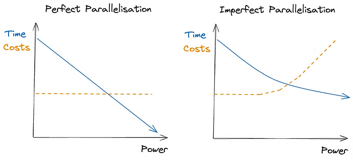
Snowflake provides many different warehouses sizes. Our pipelines can be configured to use warehouses from size XS to XL. Each size is twice as powerful as the previous one, but also twice as expensive per minute. If the query is perfectly parallelisable, it should run twice as fast and therefore cost the same.

That’s not the case for most queries though and we’ve saved thousands by playing around with warehouse sizes. In many cases, we’ve found that down-scaling reduced our costs by a good factor. Of course we need to accept that the query may take longer to run.

With perfect parallelisation the query is faster as your increase power so the costs are constant. With imperfect parallelisation the gains on the query time are more and more marginal as you increase power, so your costs ( = time * power) increase

What’s next?

First off, we’ll be following up with a post laying out the different tools that helped us identify, prioritise and track our Snowflake cost reduction efforts. And we’ll be detailing that so that you can set those up at your company too.

New tools, new rules

We’ve built some new tools during this sprint and we’ll be using them to monitor cost increases and track down the guilty pipelines.

We’ll also make sure to enforce all the good practices we’ve outlined in this post and have a link to this live somewhere in our doc for future reference.

Wait we’re underspending now?

So apparently we went a bit too hard on those cost reduction efforts and we’re now spending less credits than what we committed for in our Snowflake contract. Nobody is necessarily complaining about this “issue”…but it’s nice to know we have some wiggle room to experiment with more advanced features that Snowflake has to offer. So, we are going to do just that.

One area that could use some love is our events system. The current state involves an hourly pipeline to batch load these events into Snowflake. But, we could (and most definitely should) do better than that. Snowpipe Streaming offers a great solution for low-latency loading into Snowflake tables, and the Snowflake Connector for Kafka is an elegant abstraction to leverage the Streaming API under the hood instead of writing our own custom Java application. More to come on this in a future blog post!

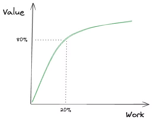
The 20/80 rule

I think this applies to this project. There’s tons of other pipelines we should investigate and we can probably get some marginal savings on each of them. But it will probably take twice as much time for half the outcome… We’ll be evaluating our priorities but I already know that there’s other areas of our backend we can focus on that will yield some bigger and quicker wins.

A poor attempt at illustrating the 20/80 rule

Modularize datasets for re-use

Although we put some effort into this already, there is certainly a lot more to do. Currently, all of our production tables live in the PUBLIC schema no matter if it’s a source or derived table, which doesn’t make discovering data very intuitive. We are exploring using the Medallion Architecture pattern to apply to our Snowflake environment for better table organization and self-service discovery of existing data. Hopefully this will lay a better foundation for modularity!